Introduction

Pipeline operation within feasible conditions could be a routine matter, while taking the operation to the optimal conditions is a task needing rigorous effort. The objective is normally concerned with maximization of profits and reducing costs, remaining within operational boundaries, maintaining the delivery targets, and at the same time adhering to existing safety criteria. The goal is to achieve the optimality of operation which runs under strict environmental and safety regulations, intense competition and narrowing profit margins.

Pipeline optimization using online simulators is gaining wide acceptance as one of the most cost-effective and reliable ways to achieve the optimal operating conditions. A well-defined pipeline model, a simulator coupled with optimization software comprises the main components of any successful scheme.

Formulation

The day-to-day operation is dictated by two main functions – safety and economy. Safety rules ensure hazard-free operation, by way of a host of operating criteria governing effluent control, capacity limits and operating thresholds. These rules form a set of operating constraints and define the boundaries for a safe operating envelope. Figure 1 is a diagram showing the coexistence of three operating environments. Within the outermost zone of possible operating conditions there is an envelope enclosing an area of safe operation.

Points inside the safe operating envelope represent the allowable operating conditions with varying profit levels. All points satisfy the safety criteria but not necessarily the economy. Our purpose is to locate the point corresponding to the highest level of profits in the optimal zone which may exist within the area of safe operation.

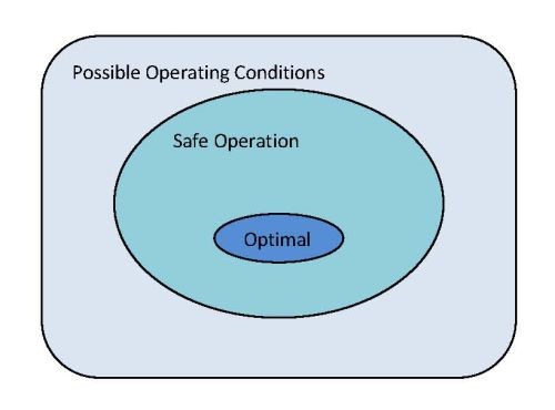
Figure 1 Different Operating environments

The mathematical formulation leads to a nonlinear constrained optimization problem. The objective function and the constraints are non-linear functions of operating variables. A statement of the general mathematical formulation is given below:

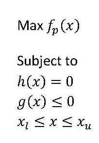
x is the vector of the state variables, representing pressures, temperatures, flow-rates and other dominant independent process variables. f_ps the objective function representing profits, which is the difference between the sales and operating costs. Since we are concerned only with the operational aspect we may well try to minimize the operating costs. The operating cost involves one major constituent, transportation energy usage and service costs. Now we can rewrite our objective as Min f_c(x) where f_c is the cost function.

h(x) represents a set of constraints attached to the modelling equations of the various unit operation devices, such as pumps, compressors, heat exchangers, and pipelines and supply and delivery conditions. Natural gas distribution network may form a cluster of hundreds of pipe sections and loops. There are multi-supply points, several interconnected pipeline networks operated at different pressure levels.

Pressure and flow at multi-supply stations, network nodal points, pressure and flow in pipe sections are state variables subject to operational and safety constraints.

g(x) are a set of inequalities, some of which are equalities, representing the safety constraints, operational restrictions and delivery quality specifications. Other constrains may be, for example, the maximum allowable working pressure, temperature of field equipment.

The x- state vector is only allowed to vary inside a feasible zone bracketed by the lower and upper bounds, denoted by two vectors x_l and x_u.

The formulation leads to a constrained nonlinear optimization problem in which the optimal vector x is searched for the conditions that returns a local minimum of the scalar function f_c(x). The solver must enwrap a solution method that must be capable of solving the multi-variable constrained non-linear optimization problem. The optimization software should have accessibility to the function values h(x) and g(x) generated by the integrated pipeline simulator.

Much advancement has been made in the field of constrained nonlinear optimization in recent times and, as a result, algorithms based on elegant methods are available. They all originate from the classical search methods and employ excellent refinements and efficient numerical techniques in seeking out a solution. Function and gradient values are calculated repeatedly from the pipeline model for the objective, constraints and their derivative functions.

The integrated optimization and pipeline simulation software can be used as a predictive model. The predictive model satisfying the desired boundary conditions can be extended to function as a look-ahead model. The look-ahead simulation normally starts from a set of state variables by setting their initial point values to those taken from a close historical profile or from a snap-shot of the current pipeline operation. The look-ahead simulation results are expected to be reasonably representative of the future state of the pipeline. The pipeline model is a mathematical approximation described by a set of state variables defining the process, but in practice the real life pipeline systems comprise other hidden dominant controlling variables that are left out from the classical mathematical model. The discrepancy between the classical and real model begins to appear as the simulation progresses when the measured field data collected from SCADA reports the violations of boundary conditions. The general pipeline simulator formulated on equation based pipelines and devices generate results that do not always match the real operation. The simulator can be brought in line with the realistic operation by suitably modifying the pipeline and device models making use of the bank of historical SCADA data values issued by the respective device.

The predictive model can be extended to the real time model in which the simulated operation is matched against measured operation and the deviations can be corrected by adjusting the state variables driving the boundary conditions to fall within limits. The altered values of state variables for the desired operation changes are generated by the pipeline simulator which includes all associated devises such as compressor stations, regulators, meters, valves. The modified values of the operation variables tune the device characteristics to match modelled operation against measured operation. The real time model operation brings about a more accurate estimation of the future state of the pipeline.

The SCADA data does not guarantee its accuracy and quality as the signal is normally acquisitioned along with noise and the data must be refined by a statistical filtration method before processing when determining the real time operation adjustments.

Application

We look at a case of cost minimization on on-shore pipeline. The pipeline carries high pressure ethylene from the production plant, over a distance of several hundred kilometres, to the processing plant where ethylene is converted into the finished products. The pipeline traverses several ranges of hills, and crosses a number of rivers and canals in the lowlands. It is composed of a number of pipe segments of different diameters. There are two compressor stations, one at the supply point and the other roughly halfway between the supply and delivery points. In addition to the compressors, the transportation scheme contains ancillary equipment such as block-valves, meters and filters.

Ethylene (C2H4) is a colourless and flammable gas and forms the most important feedstock for the petrochemical industry. During transportation the ethylene is maintained as a “dense” phase fluid, i.e. a region in the fluid’s phase diagram above the critical point (50.4 bara, 9.2⁰C). The dense phase ethylene has properties of both liquid and gas, and is heavy but compressible. Its thermodynamic properties are peculiar, in particular the density which is extremely sensitive to pressure and temperature – at 60 barg, its density can drop from 360 to 180 kg/m3 when the temperature changes from 4⁰ to 20⁰ C. Fluid density has a direct influence on the line friction loss, a characteristic resulting in the diverse pumping costs in the winter and summer operations. It therefore follows that maximum line throughput is constrained by the ambient conditions. There is another important safety constraint to be considered. Ethylene must be kept above the critical point anywhere in the pipeline, as the fluid’s behaviour in the critical region is unstable, leading to two-phase flow conditions. Liquid-gas mixtures in an undulating pipeline tend to arrange themselves with the heavy on all the up-grades and lighter on all the down-grades, creating cumulative back pressure and making flow unpredictable⁽¹⁾. It is imperative that the line pressure at the high peaks and the receiving end must be kept above the critical pressure and hence there is a necessary safety requirement that the line pressure at any point is kept above 58 barg. There are other constraints governing pressure and flow conditions at delivery points, imposed by the consumers.

The object is to minimise the total of the compressor running costs f_c given supply and delivery schedules which can be written in the generalised form as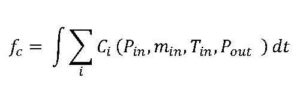where C_irepresents the running cost of the ith compressor and is a function of pressure (P), temperature (T), flow (m) at inlet conditions (in) and discharge pressure (out). Total expenditure is the sum of the running costs for all the compressors over a given time period t. The process modelling equations, h(x) =0 for the pipeline, compressors, valves and filters are handled by the pipeline simulator. The ethylene thermophysical property relationships (NBS equation of state⁽²⁾ ) also contribute to the same set of equations. Next, we state the member functions of the inequality constraints g(x)≤0. Pressure, flow and temperature profiles are known at the supply point (x=0). Delivery point (x=l) pressure and flow profiles are specified for the duration of operation τ.

P(x,t), m(x,t), T(x,t) are known for 0 ≤ t ≤ τ and x = 0.
P(x,t), m(x,t) are known for 0 ≤ t ≤ τ and x = l.

An important safety constraint is that the line operating pressure must be below the allowable design pressure and above critical pressure at any point on the line and for the whole duration, as expressed below.

P_critical < P(x,t) < P_allowable for 0 ≤ t ≤ τ and 0 ≤ x ≤ l.

This summarized mathematical statement represents the general optimization problem concerning the compressor running costs.

At this point we will restrict our analysis to a special case that arises from the steady-state conditions of a pipeline operating under a single compressor at the supply point, and look at some numerical results.

The supplier guarantees a steady flow of ethylene at 40 tonnes per hour, 75.7 barg and 10⁰C, while the delivery conditions demand a continuous delivery at 40 tonnes per hour and a pressure not less than 60 barg. The pipeline has a maximum allowable working pressure of 98 barg and the fluid pressure is not allowed to drop below 58 barg (critical pressure plus an allowance for fluctuations). With only the supply end compressor in operation we are required to determine the optimal conditions for the pipeline operation.

The constraints are now reduced to the following form:

P(x) = 75.7, m(x)=40, T(x)=10 for x = 0.
P(x)≥ 60, m(x)=40 for x = l.
58 < P(x) < 98 for 0 ≤ x ≤ l.

We notice that if a value for the compressor discharge pressure is assumed, it defines a possible operating environment that can be explicitly solved using a pipeline simulator. Since all inlet conditions are known, the compressor can be solved for the exit temperature and power consumption, for a given discharge pressure. The compressor exit stream is the inlet to the pipeline, and hence the pipeline can be completely solved to obtain its pressure profile and properties at the delivery end. The simulation results confirm whether or not the selected conditions are feasible and fall inside the safe operating envelope. It follows that the employment of the process simulator has reduced the study into a single variable optimization problem of compressor discharge pressure to minimize the running cost.

The GBST pipeline simulator linked to EPROP the ethylene thermodynamic and transport property software that uses the NBS equation of state provided function values to the optimization software which in this instance converges to solution rapidly.

Figure 2 shows the line pressure profiles under different discharge pressures of the compressor. If the compressor discharge is maintained at an arbitrary high pressure (say 85 barg), but below the maximum allowable line pressure, then we have an operation that satisfies all the constraints; we have chosen a point inside the safe operating envelope. This probably is the situation with most plant operations, where the plant managers would elect to ‘play safe’, with no available help to investigate other operating possibilities that may lead to a better decision. At 85 barg discharge pressure, the delivery pressure is close to 68 barg, which is much higher than the customer specifications, and an obvious wastage of compressor power. The optimal solution should correspond to a lower compressor power.

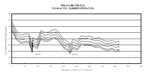
Figure 2. Effect of Compressor Discharge Pressure on Line Pressure Profile

Since compressor running cost is directly related to discharge pressure, the solution is found in the direction of decreasing values of the compressor discharge pressure. The minimum delivery pressure of 60 barg is satisfied when the compressor discharge is at 76 barg, which, in the absence of any other information, seems to suggest the most economical conditions. This operation nevertheless forces the fluid pressure to drop below 58 barg at the peaks, thus violating safety constraints. As the optimizing software scans the entire line pressure profile and detects the violation of pressure constraints the above operation is not selected as the optimum. It would rather pivot the pressure at one of the peaks to 58 barg and treat it as the limiting constraint and the search algorithm proceeds with the process.

At the solution, the optimal conditions satisfying all safety constraints are found when the Peak 2 pressure is just above 58 barg, giving a compressor discharge pressure of 79 barg and a delivery pressure of 63 barg.

Demand for higher flow rates can change the operating scenario entirely, and we may need to widen the scope of our problem definition accordingly. A higher volume throughput (say around 70 tonnes per hour) during summer causes more friction loss, making it predominant over the gravity head, the factor that would redefine the shape of the new pressure profile.

In this situation it will be more economical to bring the intermediate compressor also into operation, thus increasing the number of the state variables associated with our optimization problem. The additional state variables are needed to account for the inlet and discharge conditions of the intermediate compressor.

The formulation follows the same steps that we discussed earlier, but it includes a modified objective function and a different set of constraints. This shows that a single addition of another operating variable can bring about alteration to the process configuration, thus opening up challenging new scenarios for true multi-variable optimization.

References

1. Nolan, H.G.B., “How to handle ethylene in a pipeline-Part I”, Oil and Gas International, Vol. 9, No. 6, June 1969.
2. R.D. McCarty and R.T. Jacobsen, “An Equation of State for Fluid Ethylene”, National Bureau of Standards (NBS), US, Technical Note 1045, 1981.
3. K.G. Bandara, “Optimal Plant Operation with On-Line Simulators” – Keynote Address, Indian Institute of Chemical Engineers, Coimbatore, Proceedings of the National Symposium on Computer Applications in Chemical Engineers, December 1997.